Plotting and Equation Solving

4. Plotting and Equation Solving#

Learning Objectives

Be able to:

import libraries numpy, sympy, matplotlib;
symbolically manipulate an equation using sympy.solve();
generate x and y data for a function using numpy.linspace();
plot the x, y data using matplotlib.pyplot.plot();
add horizontal lines and text to a plot; and
use pandas read_csv to open a data file
group (aggregate) data using pandas: groupby(), sum(), mean()

You will need the following extensions:

import numpy as np
import matplotlib.pyplot as plt
import pandas as pd
from sympy.solvers import solve #for solving equations symbolically
from sympy import symbols #for solving equations symbolically

4.1. Hints for Problem 1 #

\[ \mathbf{\text{% crystallinity} = \frac{\rho_c (\rho_s - \rho_a)}{\rho_s (\rho_c - \rho_a)} * 100} \]

For this problem you will need to define a function to find the crystallinity based on the values of density as shown above. Your function should look like:

def crystallinity(density_s, density_a, density_c):
    percent_crys=   # finish this statement
    return percent_crys

crystallinity(0.925, 0.870, 0.998)  # checking your function output

Write a function that takes percent_crystallinity, crystalline_density and amorphous_density and returns the sample density. For example,

def sample_density(percent_crystallinity, density_a, density_c):  
     density_s=   #finish this equation
     return density_s

To find the equation for the sample density, you will want to solve the crystallinity equation for the sample_density. You can do this using sympy after loading the following packages:

from sympy.solvers import solve #for solving equations symbolically
from sympy import symbols #for solving equations symbolically

4.1.1. Example of solving an equation#

Let’s say you wanted to solve the equation \(a x^2 + b x + c = d\). First, we tell python that a,b,c,d,x are symbols.

from sympy.solvers import solve #for solving equations symbolically
from sympy import symbols #for solving equations symbolically

a,b,c,d,x = symbols('a b c d x')

Then we can use the solve command.

Important

The equation that goes into the solve command must equal zero so we rewrite \(a x^2 + b x + c = d\) as \(a x^2 + b x + c - d=0\). Notice that we do not include the “=0” part in the solve function below because that is assumed.

# solve for x
solve(a*x**2+b*x+c-d, x)

[(-b - sqrt(-4*a*c + 4*a*d + b**2))/(2*a),
 (-b + sqrt(-4*a*c + 4*a*d + b**2))/(2*a)]

def x_solution(a,b,c,d):
    return (-b + np.sqrt(-4*a*c + 4*a*d + b**2))/(2*a)

x_solution(2,9,5,10)

0.5

x_solution(2,9,0.4,10)

0.8904617494884413

Let’s find our x solution for different values of the parameter “d”

The np.linspace(min, max, numpts) creates evenly spaced points between two numbers. The number of points you want is given by the third number.

dd=np.linspace(0,5,5) #first pt =0, last point=5, total points=5
print('linspace list dd = ',dd)
[x_solution(2,9,5,d) for d in dd] #list comprehension loop

linspace list dd =  [0.   1.25 2.5  3.75 5.  ]

[-0.6492189406417879,
 -0.4646428928642874,
 -0.2974375810233365,
 -0.14346255670591024,
 0.0]

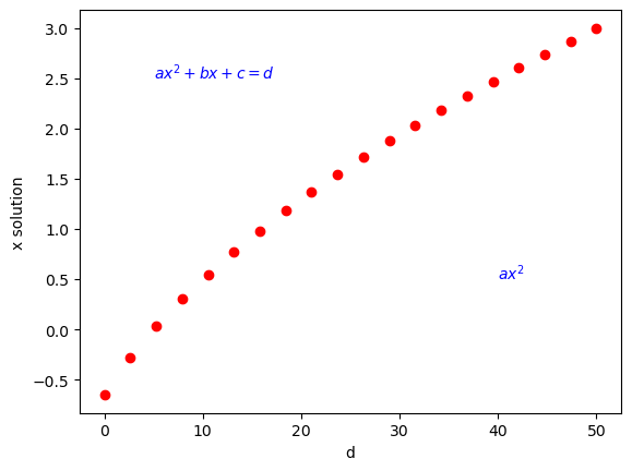
Let’s use the above method to find x solutions for 20 d values between 0 and 50. Example annotations are also included in the plot.

d=np.linspace(0, 50, 20) #creates 20 evenly spaced d-values from 0 to 50
x_sol=x_solution(2,9,5,d)
plt.plot(d,x_sol,'ro')
plt.xlabel('d')
plt.ylabel('x solution')
plt.annotate('$a x^2 + b x + c = d$', xy=(5, 2.5), color='b') # you can include text on your plot
plt.annotate('$a x^2$', xy=(40, 0.5), color='b') # you can include text on your plot
plt.show()

../_images/79d326451e8108e94901f892ac7f9f8c55b4351280280317fc52ed87c1ec2a5d.png

4.2. Hints for Problem 2 #

Last week we calculated the value of \(\left(4\times \frac{\text{pts in circle}}{\text{total num pts}}\right)\) for 1000 random points. This week you will plot the value as a function of the number of random points. That is, you want to write a function that takes a parameter, \(n\), for the total number of points and returns the value \(\left(4\times \frac{\text{pts in circle}}{\text{total num pts}}\right)\).

My code for 1000 random points was:

xcoord=(2)*np.random.random(1000)-1 #1000 random pts from -1 to 1
ycoord=(2)*np.random.random(1000)-1 #1000 random pts from -1 to 1
magnitude=np.sqrt(xcoord**2+ycoord**2) #length from center (0,0) to point
mag_test=magnitude<=1
4*len(xcoord[mag_test])/len(xcoord)

Check what len(xcoord[magnitude<=1]) and len(xcoord) does in my code above.

Since your n value in this problem will vary from 100 to 1,000,000 (i.e. several orders of magnitude) it is better to use geomspace() rather than linspace(). geomspace() gives pts spaced on a log scale which is much better when our values change by orders of magnitude.

Don’t forget that your function above requires an integer to be input so you will want to make sure geomspace() is giving you an integer or round your list to the nearest integer.

xdata=np.geomspace(100,1e6,num=50, dtype=int) #tell it to round to the closest integer dtype=int
print('geomspace: notice the nice sample of values across all magnitudes\n')
print(xdata)
# notice the increasing step size as our numbers get larger
# compare this to linspace
print('\nlinspace: notice this skips from 100 to 20506 for the first point\n')
print(np.linspace(100, 1e6, num=50, dtype=int))

geomspace: notice the nice sample of values across all magnitudes

[    100     120     145     175     212     255     308     372     449
     542     655     790     954    1151    1389    1676    2023    2442
    2947    3556    4291    5179    6250    7543    9102   10985   13257
   15998   19306   23299   28117   33932   40949   49417   59636   71968
   86851  104811  126485  152641  184206  222299  268269  323745  390693
  471486  568986  686648  828642 1000000]

linspace: notice this skips from 100 to 20506 for the first point

[    100   20506   40912   61318   81724  102130  122536  142942  163348
  183755  204161  224567  244973  265379  285785  306191  326597  347004
  367410  387816  408222  428628  449034  469440  489846  510253  530659
  551065  571471  591877  612283  632689  653095  673502  693908  714314
  734720  755126  775532  795938  816344  836751  857157  877563  897969
  918375  938781  959187  979593 1000000]

4.3. Hints for Problem 3 #

Import the csv file titanic.csv and (a) determine the percentage of woman that survived and the percentage of men that survived and (b) determine the average ticket price (Fare) for those that survived versus those that did not survive. 0 = did not survive. 1 = survived.

Last week we learned how to use pandas to import an excel file; clean imported data including dropping NAN, filling NAN, renaming columns, dropping rows, sorting, slicing, and adding new columns.

*Now we need to learn how to group (aggregate) data: groupby(), sum(), mean()
Let’s take a look at a data file containing information about the insulation thickness from a wire coat machine versus several parameters.

# This is a direct read of the file "raw_clean_cable_insulation.csv" from a google drive. 
raw=pd.read_csv('https://drive.google.com/uc?id=1zmsrtUgXZhJJzERQXFKkUVoCD1zNbBSr')
raw.head(3) #looking at only first 3 records

	Unnamed: 0.1	Unnamed: 0	ExtrTemp	LineSpeed	WaterTemp	Measure	City
0	0	0	234.83	55.28	26.67	170.67	Kairo
1	1	1	235.09	54.13	26.97	182.86	Kairo
2	2	2	235.09	54.33	27.46	182.74	Kairo

# dropping first two columns here since I don't need them
df=raw.drop(['Unnamed: 0.1','Unnamed: 0'],axis=1)
df

	ExtrTemp	LineSpeed	WaterTemp	Measure	City
0	234.83	55.28	26.67	170.67	Kairo
1	235.09	54.13	26.97	182.86	Kairo
2	235.09	54.33	27.46	182.74	Kairo
3	235.05	55.00	26.83	175.49	Kairo
4	235.04	55.26	26.62	172.80	Kairo
...	...	...	...	...	...
9992	234.92	55.09	26.98	173.84	Cairo
9993	235.22	55.91	27.30	171.86	Cairo
9994	235.13	55.43	26.99	173.59	Cairo
9995	235.05	54.73	26.73	177.21	Cairo
9996	235.10	54.57	27.21	180.25	Cairo

9997 rows × 5 columns

# rounding some of the numbers so they group better
# i.e. 234.92 and 235.22 etc should all just be 235.  
# you won't need to do this for the titanic data
df['LineSpeed']=df.loc[:,'LineSpeed'].round(1)
df['ExtrTemp']=df.loc[:,'ExtrTemp'].round(0)
df

	ExtrTemp	LineSpeed	WaterTemp	Measure	City
0	235.0	55.3	26.67	170.67	Kairo
1	235.0	54.1	26.97	182.86	Kairo
2	235.0	54.3	27.46	182.74	Kairo
3	235.0	55.0	26.83	175.49	Kairo
4	235.0	55.3	26.62	172.80	Kairo
...	...	...	...	...	...
9992	235.0	55.1	26.98	173.84	Cairo
9993	235.0	55.9	27.30	171.86	Cairo
9994	235.0	55.4	26.99	173.59	Cairo
9995	235.0	54.7	26.73	177.21	Cairo
9996	235.0	54.6	27.21	180.25	Cairo

9997 rows × 5 columns

Let’s find the percentage of Measurements made in Alexandria vs the total number of measurements.
Let’s also find the average WaterTemp for all measurements made in Alexandria at an ExtrTemp of 235.0

# groupby collects all records for the different cities and then
# .count() counts how many records there are in each city grouping
dfgroup=df.groupby(['City']).count()
dfgroup

	ExtrTemp	LineSpeed	WaterTemp	Measure
City
Alexandria	5520	5520	5520	5520
CAI	17	17	17	17
Cairo	4413	4413	4413	4413
Kairo	47	47	47	47

# using .sum() we can get the total number of records in each column
# by default .sum() sums down columns
dfgroup.sum()

ExtrTemp     9997
LineSpeed    9997
WaterTemp    9997
Measure      9997
dtype: int64

# calculating percent of records in Alexandria vs total of 9997
# using .loc[] to pull from dataframe "dfgroup.loc[row, column]"
dfgroup.loc['Alexandria','Measure']/9997*100 #percent

55.21656496949085

# now we are grouping by two columns
# we first collect the Cities
# then group within each city by the ExtrTemp (extruder temperature)
# here we take the mean or average value in these two categories for each column
dfmean=df.groupby(['City','ExtrTemp']).mean()
dfmean

		LineSpeed	WaterTemp	Measure
City	ExtrTemp
Alexandria	234.0	54.894118	27.056471	170.712353
	235.0	55.003924	26.999927	175.425584
	236.0	55.115152	27.000606	180.169091
CAI	235.0	55.176471	26.965882	174.288235
Cairo	234.0	54.980645	27.035806	169.769032
	235.0	54.994089	26.993054	175.444202
	236.0	55.014706	27.005294	181.228824
Kairo	235.0	55.093617	26.941915	174.370426

# the mean value of WaterTemp in Alexandria at an ExtrTemp of 235 degrees is
# note row is ('Alexandria',235.0) and the column we want is 'WaterTemp'
dfmean.loc[('Alexandria',235.0), 'WaterTemp']

26.999926645883

4.3.1. Pivot Table#

For a lot more control, we could use pivot_table to specify different aggregation functions for each column of values we want to analyze. You should be able to do what you want with groupby() but the pivot_table is a more manual way to specify many options.

pd.pivot_table(df, values=['Measure', 'WaterTemp','LineSpeed'], index=['City', 'ExtrTemp'],
                    aggfunc={'Measure': np.mean,
                             'WaterTemp': [min, max, np.mean],
                            'LineSpeed':[np.sum,np.mean,np.size]}).style

		LineSpeed			Measure	WaterTemp
		mean	size	sum	mean	max	mean	min
City	ExtrTemp
Alexandria	234.000000	54.894118	34	1866.400000	170.712353	27.560000	27.056471	26.520000
	235.000000	55.003924	5453	299936.400000	175.425584	27.700000	26.999927	26.150000
	236.000000	55.115152	33	1818.800000	180.169091	27.440000	27.000606	26.420000
CAI	235.000000	55.176471	17	938.000000	174.288235	27.330000	26.965882	26.440000
Cairo	234.000000	54.980645	31	1704.400000	169.769032	27.410000	27.035806	26.580000
	235.000000	54.994089	4348	239114.300000	175.444202	27.660000	26.993054	26.290000
	236.000000	55.014706	34	1870.500000	181.228824	27.300000	27.005294	26.700000
Kairo	235.000000	55.093617	47	2589.400000	174.370426	27.460000	26.941915	26.380000

4.4. Exercises#

4.4.1. Problem 1:#

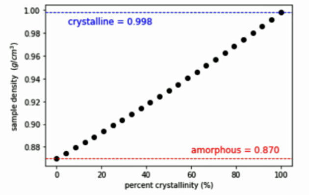
Computations of the Density and Percent Crystallinity of Polyethylene (Callister 10th ed., section 14.11)

The % crystallinity is given by:

\[ \mathbf{\text{% crystallinity} = \frac{\rho_c (\rho_s - \rho_a)}{\rho_s (\rho_c - \rho_a)} * 100} \]

(1) Write a function that calculates the percent crystallinity of a branched polyethylene sample \(\rho_s\) that has a density of \(0.925\ 𝑔\ 𝑐𝑚^{-3}\) . The density of a totally amorphous material \(\rho_a\) is \(0.870 \ 𝑔\ 𝑐𝑚^{-3}\) and the density of a totally crystalline \(\rho_c\) material is \(0.998 \ 𝑔\ 𝑐𝑚^{-3}\) .

(2) Calculate the sample density \(\rho_s\) versus % crystallinity and reproduce the plot below (including the horizontal lines and text). To find the equation for the sample density use the solve commands from sympy to solve the above crystallinity equation for \(\rho_s\). An example of using solve can be found in this lesson.

(3) Export your data to an excel file.

4.4.2. Problem 2:#

Write a function that finds “x” random points in a square of edge length 2 centered at (0,0). Determines how many of these points are contained in a circle of radius 1 centered at (0,0). Returns the value \(\left(4\times \frac{\text{pts in circle}}{\text{total num pts}}\right)\). Plot the value \(\left(4\times \frac{\text{pts in circle}}{\text{total num pts}}\right)\) versus number of points, x. Your x should vary between 100 and 1e6. Also include a horizontal line at the value of pi on your plot.

4.4.3. Problem 3:#

Import the csv file “titanic.csv” and (a) determine the percentage of woman that survived and the percentage of men that survived and (b) determine the average ticket price (Fare) for those that survived versus those that did not survive. 0 = did not survive. 1 = survived.

Plotting and Equation Solving

Contents