3. Short Lesson: Plotting Basics

From: https://matplotlib.org/3.1.1/tutorials/introductory/pyplot.html#sphx-glr-tutorials-introductory-pyplot-py

3.1. Plotting basics

# only need to import these once
# place all import statements in the first cell of your notebook
import numpy as np
import matplotlib.pyplot as plt

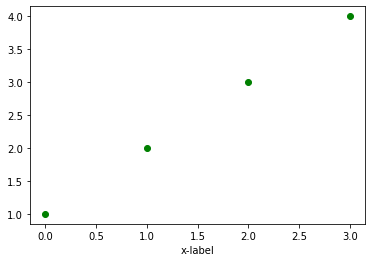
# instead of bo, try b^ or bs
# instead of b try r or g
plt.plot([1, 2, 3, 4], 'go')
plt.xlabel('x-label')
plt.show()

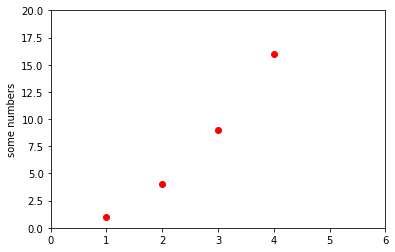
plt.plot([1, 2, 3, 4], [1, 4, 9, 16], 'ro')
plt.ylabel('some numbers')
plt.axis([0, 6, 0, 20])
plt.show()

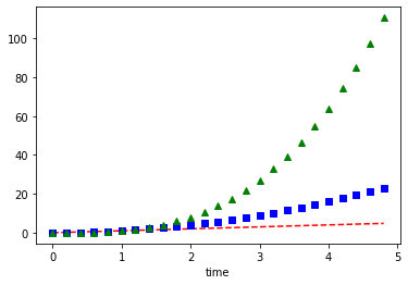
# evenly sampled time at 200ms intervals
t = np.arange(0., 5., 0.2)

# red dashes, blue squares and green triangles
plt.plot(t, t, 'r--', t, t**2, 'bs', t, t**3, 'g^')
plt.xlabel('time')
plt.show()

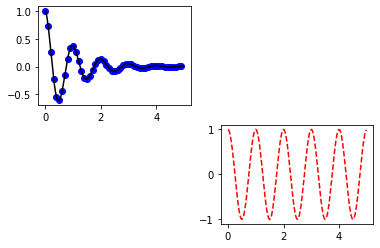
def f(t):
    return np.exp(-t) * np.cos(2*np.pi*t)

t1 = np.arange(0.0, 5.0, 0.1)
t2 = np.arange(0.0, 5.0, 0.02)

plt.figure()
plt.subplot(221)
plt.plot(t1, f(t1), 'bo', t2, f(t2), 'k')

# 224 = 2 rows, 2 col index 4 is low-right 
# count across then down i.e. index 1 is upper-left
plt.subplot(224)
plt.plot(t2, np.cos(2*np.pi*t2), 'r--')
plt.show()