4. Short Lesson: Plotting functions

# only need to import these once
# place all import statements in the first cell of your notebook
import numpy as np
import matplotlib.pyplot as plt
from scipy import special #this contains the erf() function

np.e

2.718281828459045

np.exp(1)

2.718281828459045

np.linspace(-2.5, 2.5, 5)

array([-2.5 , -1.25,  0.  ,  1.25,  2.5 ])

np.arange(-2.5, 2.5, 0.5)

array([-2.5, -2. , -1.5, -1. , -0.5,  0. ,  0.5,  1. ,  1.5,  2. ])

4.1. useful functions in numpy and scipy.special

np.piecewise(x, [x < 0, x >= 0], [-1, 1])
np.linspace(-2.5, 2.5, 6)
np.log()
np.log10()
np.sin()
np.amax()
special.erf()

np.eye(2)

array([[1., 0.],
       [0., 1.]])

x=np.array([-10, -5, 0, 10])
np.piecewise(x, [x < 0, x==0, x > 0], [-1, 0, 1])

array([-1, -1,  0,  1])

x=np.array([-10, -5, 0, 10])
np.piecewise(x, [x < 0, x >= 0], [lambda x: -x, lambda x: x])

array([10,  5,  0, 10])

np.linspace(-2.5, 2.5, 6)

array([-2.5, -1.5, -0.5,  0.5,  1.5,  2.5])

np.arange(0.0, 1.0, 0.25)

array([0.  , 0.25, 0.5 , 0.75])

np.inf
np.nan
np.e
np.pi

3.141592653589793

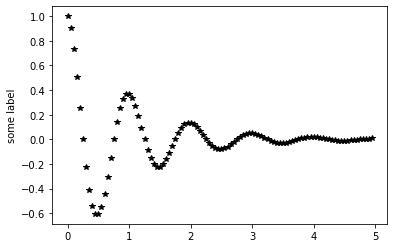
# t must be an np array not a python list
def myfunc(t):
    return np.exp(-t) * np.cos(2*np.pi*t)

xdata=np.arange(0.0, 5.0, 0.05)
ydata=myfunc(xdata)

plt.plot(xdata, ydata, 'k*')
plt.ylabel('some label')
plt.show()

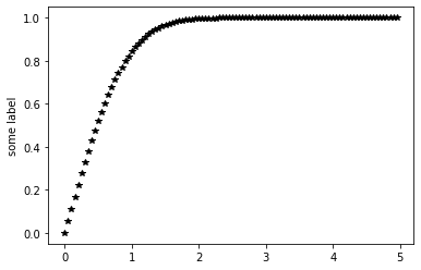
# t must be an np array not a python list
def myfunc(t):
    return special.erf(t)

xdata=np.arange(0.0, 5.0, 0.05)
ydata=myfunc(xdata)

plt.plot(xdata, ydata, 'k*')
plt.ylabel('some label')
plt.show()

4.2. Problem 17.32 Callister 10th ed. Metal oxidation.

---

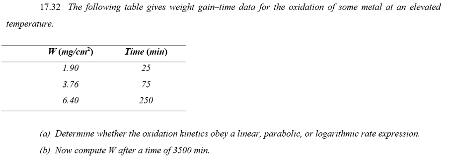
Growth laws for oxides on metals:

1. Parabolic Growth: $W^2 =K_1 \ t + K_2$
2. Linear Growth: $W = K_3 \ t$
3. Logarithmic Growth: $W=K_4\ \log(K_5\ t + K_6)$

---

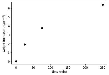
xdata=np.array([0,25, 75, 250])
ydata=np.array([0,1.9, 3.76, 6.4])

plt.plot(xdata, ydata, 'ko')
plt.ylabel('weight increase ' + r'$( mg/cm^2 )$')
plt.xlabel('time (min)')
plt.show()

from numpy import exp, linspace, random

def gaussian(x, amp, cen, wid):
    return amp * exp(-(x-cen)**2 / wid)

from scipy.optimize import curve_fit

x = linspace(-10, 10, 101)
y = gaussian(x, 2.33, 0.21, 1.51) + random.normal(0, 0.2, x.size)

init_vals = [1, 0, 1]  # for [amp, cen, wid]
best_vals, covar = curve_fit(gaussian, x, y, p0=init_vals)
print('best_vals: {}'.format(best_vals))

best_vals: [2.3458706  0.16301304 1.36857763]